Fluid Properties

1. Fluid Properties#

1.1. Density#

The density \(\rho\) of a fluid is the mass of the fluid per unit volume:

\[\rho = \frac{m}{V}.\]

Density is a point property in the sense that to get mass we have to multiply \(\rho\) by some volume. If the density is spatially uniform, we have \(m=\rho V\). For a differential volume element \(dV\), we have \(dm = \rho dV\), and the mass over some finite volume can be evaluated by integration:

(1.1)#\[m = \int_V \rho(\mathbf{x})dV.\]

In using the density this way in Eq. (1.1), we are implicitly assuming the contiuum assumption holds. That is, all spatial variations in the density are at scales much larger that molecular sizes and spacings. For example, air is mostly nitrogen \(\ce{N2}\) which has a kinetic diameter of 3.64E-10 m. In nitrogen gas at 298 K and 1 atm, there are 2.46E25 molecules per m\(^3\). This gives a distance between molecules of approximately 34E-10 m. The distance between molecules is about ten times the size of the molecules. These distances are usually much smaller than flow scales in a fluid, so we assume the fluid is a continuum, without explicitly considering its molecular structure. In liquids, the intermolecular spacing is even smaller, and is similar to the molecular size.

1.1.1. Units#

Common units of \(\rho\) are

kg/m\(^3\)
lbm/ft\(^3\)

Example: water density#

Think about an experiment you could perform to measure the density of water. What equipment would you need? How would you do it? What calculations would you do? What equation would be used? How would you know if you are right?

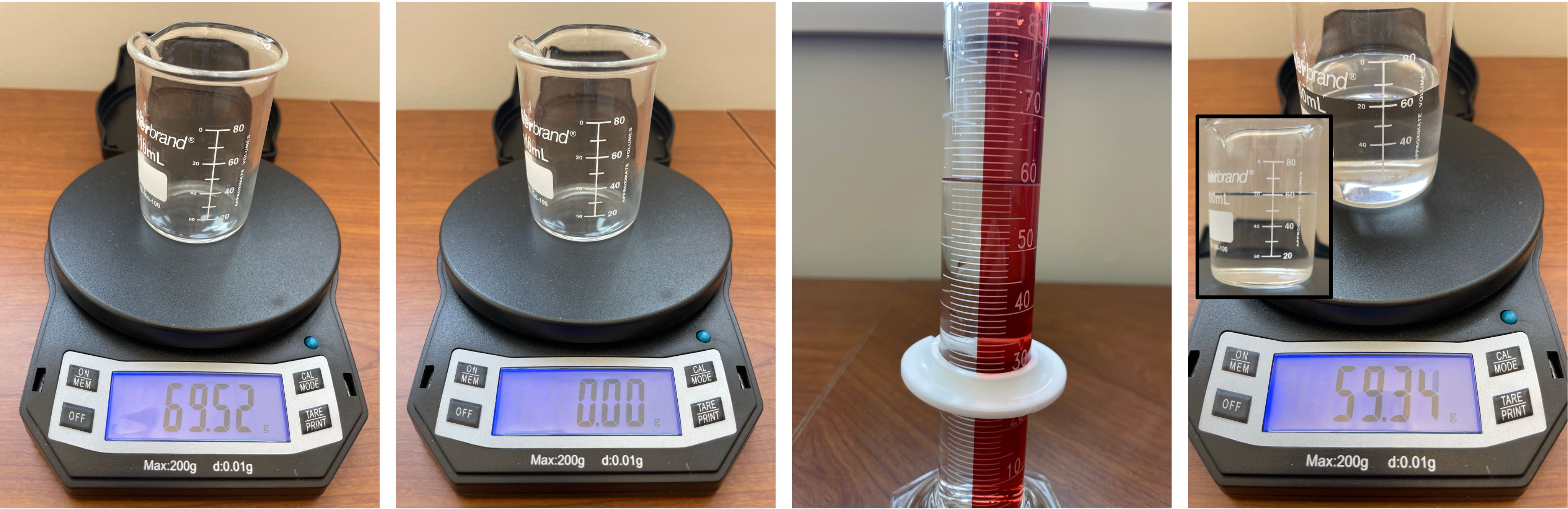
Measure the mass and volume of water. Then the density is \(\rho = m/V\).

In the image, the beaker is placed on the scale. Then we press the tare button to reset the scale to zero. A graduated cylinder is used to measure V=60 ml of water. This is added to the beaker and we measure the mass to be m=59.34 g. The density is then

\[\rho = \frac{59.34\, \mathrm{g}}{60\, \mathrm{ml}} = 0.989\,\mathrm{g/ml} = 989\,\mathrm{kg/m}^3=61.7\,\mathrm{lbm/ft}^3\]

This is compared to the literature value of 998 kg/m\(^3\) at 70 \(^o\)F. The difference is due to experimental error: error in the scale and visual error in computing the volume. The relative error is (989-998)/998 * 100% = -0.9%.

Example: particle density and bulk density of sand#

Think about an experiment to measure the density of sand. How is this different than measuring the density of water? What can you do to account for these differences?

Sand particles form a collection that is porous with many air spaces between the sand particles. We can define two densities:

the particle or material density is the density of a single particle.
the bulk density is the density of the combined sand/air mixture.

Consider the particle density. It would be very hard to accurately measure the density of a single particle because it is so small. The average particle density could be measured as \(\rho=m_s/V_s\), where \(m_s\) is the mass of just the sand and \(V_s\) is the volume of just the sand in a sand/air mixture.

The mass of just the sand is probably very close to the mass of the sand/air mixture because we expect the air to weigh much less than the sand, probably within our measurement error.
For the volume, we have \(V_\mathrm{total}=V_\mathrm{s}+V_\mathrm{a}\). We can measure the total volume, then add a known volume of water to displace the air—until the water just covers the sand after mixing it up and letting it settle.

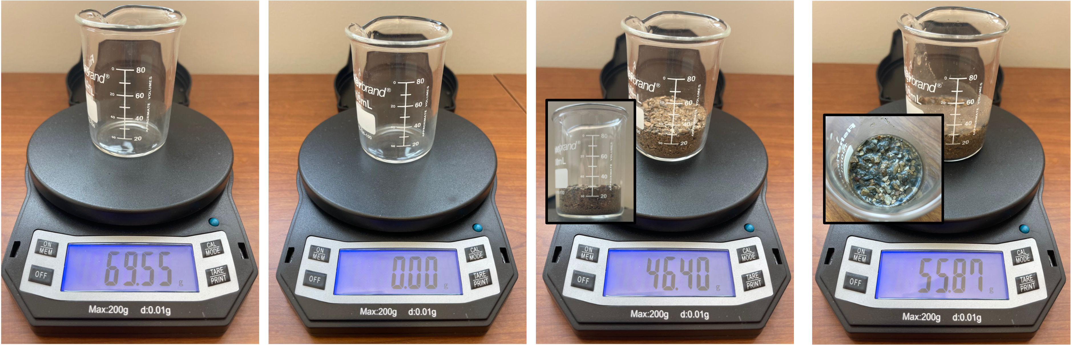
In the image, we place the beaker on the scale, then tare to 0.0, then add 30 ml of sand which shows a mass of 46.4 g, then add water to just cover the sand. The volume of water added is the mass of water added (computed by difference) divided by the density of water, as computed in the previous example.

\[m_s = 46.40 \,\mathrm{g}.\]

\[V_a = V_w = \frac{m_w}{\rho_w} = \frac{55.87-46.40\,\mathrm{g}}{0.989\,\mathrm{g/ml}} = 9.575\,\mathrm{ml}.\]

\[V_s = 30 - 9.575\,\mathrm{ml} = 20.425\,\mathrm{ml}.\]

\[\rho_s = \frac{m_s}{V_s} = \frac{46.40\,\mathrm{g}}{20.425\,\mathrm{ml}} = 2.3\,\mathrm{g/ml}=2300\,\mathrm{kg/m}^3.\]

This is the particle density. The bulk density \(\rho_b\) is

\[\rho_b = \frac{m_s}{V_\mathrm{total}} = \frac{46.40\,\mathrm{g}}{30\,\mathrm{ml}} = 1.5\,\mathrm{g/ml}=1500\,\mathrm{kg/m}^3.\]

1.1.2. Ideal gases#

The ideal gas law is commonly written as \(PV = nR_gT\). We rearrange this to \(n/V = P/R_gT\), which is moles per volume. Multiplying both sides by the mean molecular weight M of the gas gives

\[\rho = \frac{MP}{R_gT}.\]

Here, \(M\) is the mean molecular weight of the gas, \(P\) is the absolute pressure, \(R_g\) is the gas constant, and \(T\) is the absolute temperature (kelvin or Rankine).

Example: air density#

Compute the density of air at P=1 atm and 20 \(^o\)C=68 \(^oF\).

Use the given formula for the density of an ideal gas. We need to use consistent units. P=1 atm = 101325 Pa = \(\mathrm{kg/m}\,\mathrm{s}^2\). The temperature is 20 \(^oC\) = 20+273.15 K = 298.15 K, and R\(_g\)=8314.46 J/(kmol K) = (kg m\(^2\)/s\(^2\))/(kmol K). \(M\) is computed from its components as

\[M = \sum_ix_iM_i,\]

where \(x_i\) is the mole fraction of component \(i\) and \(M_i\) is the molecular weight of component \(i\). Dry air contains approximatly 78% \(\ce{N2}\), 21% \(\ce{O2}\), and 1% \(\ce{Ar}\) by mole, and these components have molecular weights of 28.0, 32.0, and 39.9, respectively. This gives M=29.0 kg/kmol. The density is then

\[\begin{split}\rho_a = \frac{(29.0\,\mathrm{kg/kmol})(101325\,\mathrm{kg/m}\,\mathrm{s}^2)}{(8314.46\, \mathrm{kg}\,\mathrm{m}^2/\mathrm{s}^2\,\mathrm{kmol}\,\mathrm{K})(298.15\,\mathrm{K})} \\ =1.18\,\mathrm{kg}/\mathrm{m}^3.\end{split}\]

Table Table 1.1 gives densities for several fluids. Note that the difference in density between air and water is nearly a factor of one thousand. This allows important assumptions and simplifications in some calculations. This is illustrated in Fig. 1.1

Table 1.1 Densities and specific gravities of several fluids.#
Fluid	\(\rho\) (kg/m\(^3\))	\(\rho\) (lbm/ft\(^3\))	SG
water (20 \(^o\)C, 1 atm)	998.19	63.3	0.998
ethanol (20 \(^o\)C, 1 atm)	789.4	49.28	0.7894
mercury (20 \(^o\)C, 1 atm)	13600	849	13.6
air (20 \(^o\)C, 1 atm)	1.204	0.07516	0.001204
CO\(_2\) (20 \(^o\)C, 1 atm)	1.830	0.1142	0.001830

../../_images/fig_air_water_vol_comparison.svg — Fig. 1.1 Relative volumes of air and water for equal masses.#

1.1.3. Specific gravity#

Specific gravity is density divided by a reference density, usually water at 4 \(^o\)C which has a density of 1000 kg/m\(^3\). That is

(1.2)#\[SG = \frac{\rho}{\rho_\text{H2O}}\]

So, a material with a specific gravity of 1 has the same density as water. A material with a specific gravity of 5 has a density five times that of water. Table Table 1.1 shows SG values for several common fluids.

1.2. Viscosity#

The viscosity \(\mu\) of a fluid is a measure of the resistance to flow. Higher viscosity fluids have higher flow friction and are more resistant to deformation. Honey has a high viscosity compared to water. See Fig. 1.2 for a simulation illustrating two fluids of different viscosities.

../../_images/Viscosities.gif — Fig. 1.2 Demonstration of flow of fluids with low (left) and high (right) viscosities. Attribution: Synapticrelay, CC BY-SA 4.0, no changes.#

Viscosity is precisely defined for a Newtonian fluid which obeys the relation

(1.3)#\[\tau = -\mu\frac{du}{dy}.\]

Here, \(\tau\) is the shear stress, \(u\) is a velocity, and \(y\) is a directional coordinate. Viscosity is a property of the fluid and depends on the fluid temperature, pressure, and composition. For Newtonian fluids, the visocity does not depend on the shear rate \(du/dy\). These quantities are illustrated in Fig. 1.3. The figure illustrates the flow between infinite parallel plates where the lower plate is fixed and the upper plate moves at some velocity \(u\). This is a so-called Couette flow.

../../_images/fig_couette_plates.svg — Fig. 1.3 Illustration of steady flow between infinite parallel plates for a Newtonian fluid.#

A linear \(u(y)\) profile is established between the plates. The shear stress \(\tau\) is the force per unit plate area required to maintain the flow, and Eq. (1.3) shows that \(\mu\) is a proportionality constant between \(\tau\) and the so-called strain rate \(du/dy\). Eq. (1.3) can be rewritten in terms of the force on the plates as

\[ F = \tau A = -\mu A\frac{du}{dy}. \]

Questions:

For a given plate area and a given \(\mu\), if we double the velocity, what happens to \(du/dy\) and the resultant force \(F\)?
If we double \(A\), what happens to \(F\), all else being equal?
If we double \(\mu\), what happens to \(F\), all else being equal?

Note, the forces involved here are frictional, that is, the force of friction due to the moving fluid. This can be described in terms of molecular collisions between faster moving fluid molecules at higher \(y\) being slowed by interactions with slower moving molecules at lower \(y\).

1.2.1. \(\tau\) is a momentum flux#

From Newton’s second law, we have \(F=ma\), or, for constant \(m\) and \(a=dv/dt\), \(F=d(mv)/dt\). Since \(mv\) is momentum, the force is a rate of change of momentum. Then \(F/A = \tau\) is a rate of change of momentum per unit area. That is, \(\tau\) is a momentum flux. We can write

\[\tau = -\mu\frac{du}{dy},\]

as an equation for momentum flux. This can be compared to conductive heat flux and diffusive mass flux, which have similar equations. In the Couette flow above, if we take \(u\) to be in the positve direction as shown, then \(du/dy\) is positive and \(F\) will be negative. The fluid exerts a negative force to the lefft on the plate, which is balanced by the external force pulling the plate to the right.

1.2.2. Units#

The units of \(\mu\) are

kg/(m\(\cdot\)s) = Pa\(\cdot\)s (SI units).
lbm/(ft\(\cdot\)s) (US units).
poise (P) or centipoise (cP), with 1 P = 0.1 Pa\(\cdot\)s, and 1 cP = 0.001 Pa\(\cdot\)s

1.2.3. Kinematic viscosity#

The viscosity \(\mu\) discussed above is called the dynamic viscosity. The kinematic viscosity \(\nu\) is frequently used, and this is simply the dynamic viscosity divided by the density:

\[\nu = \frac{\mu}{\rho}.\]

\(\nu\) has units of m\(^2\)/s, or ft\(^2\)/s.

Table Table 1.2 shows a list of dynamic and kinematic viscosities for several fluids. Note the large difference between the gases (air and CO\(_2\)) and the liquids, with the liquids having much higher dynamic viscosities, but smaller kinematic viscosities.

Table 1.2 Viscosities of several fluids.#
fluid	\(\mu\) (Pa\(\cdot\)s)	\(\mu\) (lbm/ft\(\cdot\)s)	\(\nu\) (m\(^2\)/s)	\(\nu\) (ft\(^2\)/s)
water (20 \(^o\)C, 1 atm)	1.0016E-3	6.7304E-4	1.0034E-6	1.0800E-5
ethanol (20 \(^o\)C, 1 atm)	1.1841E-3	7.9568E-4	1.5000E-6	1.6146E-5
mercury (20 \(^o\)C, 1 atm)	1.552E-3	10.43E-4	0.11412E-6	0.12284E-5
air (20 \(^o\)C, 1 atm)	1.83E-5	1.23E-5	1.52E-5	1.64E-4
CO\(_2\) (20 \(^o\)C, 1 atm)	1.47E-5	0.988E-5	0.803E-5	0.865E-4

1.3. Surface tension#

Liquids are held together by cohesive intermolecular forces. At a fluid interface these forces are nonuniformly distributed. This happens because the forces at the fluid interface are different in directions into the fluid, out of the fluid, and along the interface. These forces can make the fluid behave as if it has a skin.

../../_images/surface_tension.svg — Fig. 1.4 Illustration of molecular forces in a fluid at a surface.#

Consider a water-air interface illustrated in Fig. 1.4. Molecules in the interior of the fluid are pulled in all directions equally by attractive forces with other molecules. But at the fluid surface, the water molecules are only pulled along the surface and into the bulk fluid, (with negligible interactions between the water and air). These forces are the reason water droplets tend to form spheres: the attraction into the center deforms the fluid to minimize the surface area.

At a fluid-solid interace, the fluid will experience adhesive forces. The balance between the cohesive fluid forces and the adhesive fluid-solid forces results in interesting behavior. Water that is poured slowly from a glass will sometimes adhere to the surface and run down the side. These forces result in a meniscus when measuring liquid volumes in a graduated cylinder. When the adhesive forces are greater than the cohesive forces, the liquid climbs the sides of the glass and forms a concave surface. Otherwise a convex surface forms. See Fig. 1.5.

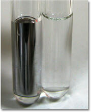
../../_images/meniscus.jpeg — Fig. 1.5 Mercury (left) with convex meniscus, and water (right) with a concave meniscus. Attribution: usgs.gov, CC BY-SA 2.0, no changes.#

Adhesive forces between a fluid and a surface give rise to capilary action in which a fluid can climb up a surface to a height where the adhesive forces balance the weight of the fluid.

Surface tension is defined a force per unit length

\[\sigma = \frac{F}{L}.\]

In Fig. 1.6, the surface tension forces balance the gravitational weight of the droplet \(F\) and \(L=\pi D\).

../../_images/droplet.svg — Fig. 1.6 Surface tension forces (white) balancing the weight of a droplet (black).#

1.3.1. Example: water surface forces#

The surface tension of water at 20 \(^o\)C is 0.07275 N/m = 72.75 dyne/cm. Surface forces are usually only important at relatively small scales. Demonstrate this by computing the diameter of a sphere of water for which the weight of the sphere equals the surface forces around the circumference of the spere.

The weight is given by

\[W = mg = \rho_wVg = \rho_w\frac{\pi}{6}D^3g.\]

The surface forces are

\[F_s = \sigma L = \sigma\pi D.\]

Equating these forces and solving for \(D\) gives

\[D = \sqrt{\frac{6\sigma}{\rho_w g}} = \sqrt{\frac{(6)(0.07275\;\mathrm{N/m})}{(998\;\mathrm{kg/m}^3) (9.81\; \mathrm{m/s}^2)}} = 0.00668\;\mathrm{m}=6.68\;\mathrm{mm}.\]

A sphere of water the size of a golf ball would have a weight 41 times higher than the surface tension multiplied by the circumference.

1.4. Pressure#

Pressure is an important property in fluid mechanics. Pressure is a force per unit area normal to a surface

\[P = \frac{F}{A}.\]

The SI unit of pressure is Pascal (Pa), with Pa \(\equiv\) N/m\(^2\). In U.S. Customary Units (USCU), pressure is given by pounds-force per square inch (psi). Note that pressure is a scalar quantity, not a vector, so the force \(F\) in the above equation represents the magnitude of the force normal to the surface.

Pressure is easier to define and visualize in terms of the force on a surface, but pressure exists throughout a fluid without a physical surface present. We can consider two adjacent fluids with an imaginary plane between them. The fluid on one side exerts a force on the adjacent fluid in the same way that the fluid exerts a force on a solid surface. This arises from molecular collisions in the fluid. The fluid-fluid interactions are the same regardless of how the plane is oriented because the molecular motions at a point don’t have any preferred direction. We say, then, that the pressure is isotropic, that is, independent of direction. This is consistent with the pressure being a scalar instead of a vector.

../../_images/pressure_collisions.svg — Fig. 1.7 Pressure on surfaces arising from molecular collisions. Attribution: Becarlson, CC BY-SA 3.0, no changes.#

Pressure, arising from molecular motions, depends on the speed of individual molecules and the rate of collisions. For ideal gases, the pressure is given by

\[P = \frac{nRT}{V},\]

where \(n\) is moles, \(R\) is the universal gas constant, \(T\) is absolute temperature, and \(V\) is volume. \(n/V\) is a molar density or concentration, which is proportional to the number of molecules per unit volume. The molecular speed is proportional to temperature. Hence, the pressure increases as both the molecular speed increases, and as the concentration of molecules increases. That is, pressure is higher when the molecules strike “harder” and strike more often.

In general, the pressure in a fluid changes from one location to another, and depends on fluid velocity and the depth of the fluid. The effect of fluid depth is discussed in Fluid Statics.